9.2. Flux Limiters

This chapter is co-written with Sigrid Christine Pedersen (student in GEOF211 spring 2025)

The minmod limiter, described in chapter Min-mod limiters is useful to avoid strong slopes for the reconstructed signal. Using flux limiters, is another approach to gain controll over the model behaviour near strong gradients. To understand the flux limiters, we must first look into how numerical schemes can be written in a flux form:

The flux form of the advection scheme can be written:

(9.8)\[q_k^{n+1}=q_k^n+\frac{\Delta t}{\Delta x}[F_{k-1/2}^n-F_{k+1/2}^n]\]

The flux form means that we split up what is entering the grid cell \(k\) from the left, \(F_{k-1/2}^n\) (entering from grid cell \(k-1\)), and what is leaving the grid cell towards the right \(F_{k+1/2}^n\) (leaving from grid cell \(k\)).

Note

The Advection equation on the flux form looks very similar to the simple schemes, such as the FTBS, FTBS, or FTCS. But, note that the sign in front of \(\frac{\Delta t}{\Delta x}\) is positive and that the advection speed \(a\) is included in the fluxes. The sign is positive, since we do the flux from the left minus the flux from the right inside the paranthesis.

9.2.1. Godunov on Flux form

We can write the Godunov scheme on Flux form by identifying terms related to grid cell \(k-1\) and grid cell \(k\). If we repeat the Godunov step 2 equation with colors to help us separate the terms, we get:

(9.9)\[q_k^{n+1} = {\color{Cerulean}{q_k^n}} - a {\color{Cerulean}{\frac{\Delta t}{\Delta x}}} \left( {\color{teal}{q_k^n}} - {\color{salmon}{q_{k-1}^n}} \right) - \frac{a \Delta t}{2} \left( 1 - \frac{a \Delta t}{\Delta x} \right) \left( {\color{teal}{\sigma_k^n}} - {\color{salmon}{\sigma_{k-1}^n}} \right)\]

(9.10)\[{\color{Cerulean}{q_k^{n+1}}}={\color{Cerulean}{q_k^n}}+\frac{\Delta t}{\Delta x}[F_{k-1/2}^n-F_{k+1/2}^n],\]

where

(9.11)\[\begin{split}\begin{aligned} {\color{salmon}{F_{k-1/2}^n}}&=a{\color{salmon}{q_{k-1}^n}}+\left(\frac{\Delta x}{2}-a\frac{\Delta t}{2}\right)a{\color{salmon}{\sigma_{k-1}^n}}\\ {\color{teal}{F_{k+1/2}^n}}&=a{\color{teal}{q_{k+1}^n}}+\left(\frac{\Delta x}{2}-a\frac{\Delta t}{2}\right)a{\color{teal}{\sigma_{k+1}^n}} \end{aligned}\end{split}\]

Now that we have the advection equation on the flux form, we can define a flux limiter \(\phi(\theta)\) to avid overshoots and undershoots near strong gradients or local maxima and minima of the signal \(q(x,t)\). Here, \(\theta\) is a smoothness indicator, defined as

where

(9.12)\[\theta_{k+1/2}^n=\frac{q_k^n-q_{k-1}^n}{q_{k+1}^n-q_k^n}\]

From equation (9.12), we can note a few details:

• \(\theta\) is defined at the grid cell edge \(k+1/2\).

• The nominator and denominator contains a backward (upwind) and a forward (downwind) difference of \(q_k^n\), respectively.

• If \(\theta\) is positive, the upwind and the downwind slopes have the same sign and \(q_k^n\) is not a local extremum.

• If \(\theta\sim+1\), the upwind and downwind slopes are similar, indicating similar behavior of the signal for the neighboring points

• If \(\theta\) is negative, the upwind and downwind slopes have different signs and \(q_k^n\) is a local extremum that may require action to avoid overshoots and undershoots

The flux limiter \(\phi(\theta)\) takes on a value for each grid cell, based on the value of \(\theta\).

Note

You can think of the flux limiter as some kind of switch, or an if statement in coding. When you code up a flux limiter, you check the value of \(\theta\) for each grid cell, and then define a value \(\phi(\theta)\) for each grid cell.

The Godunov fluxes from (9.11) with limiters, will now look like:

(9.13)\[\begin{split}\begin{aligned} F_{k-1/2}^n&=aq_{k-1}^n+\left(\frac{\Delta x}{2}-a\frac{\Delta t}{2}\right)a\sigma_{k-1}^n\phi(\theta_{k-1/2}^n)\\ F_{k+1/2}^n&=aq_{k+1}^n+\left(\frac{\Delta x}{2}-a\frac{\Delta t}{2}\right)a\sigma_{k+1}^n\phi(\theta_{k+1/2}^n) \end{aligned}\end{split}\]

If we, as an example, choose the downwind slope \(\sigma_k^n = \frac{q_{k+1}^n - q_k^n}{\Delta x}\), the full set of equtions for the Godunov advection scheme on flux form with limiters become:

(9.14)\[\begin{split}\begin{aligned} q_k^{n+1} & =q_k^n+\frac{\Delta t}{\Delta x}[F_{k-1/2}^n-F_{k+1/2}^n]\\ F_{k-1/2}^n & =aq_{k-1}^n+\left(\frac{\Delta x}{2}-a\frac{\Delta t}{2}\right)a\frac{q_{k}^n - q_{k-1}^n}{\Delta x}\phi(\theta_{k-1/2}^n)\\ F_{k+1/2}^n & =aq_{k+1}^n+\left(\frac{\Delta x}{2}-a\frac{\Delta t}{2}\right)a\frac{q_{k+1}^n - q_k^n}{\Delta x}\phi(\theta_{k+1/2}^n) \end{aligned}\end{split}\]

\(C=a\frac{\Delta t}{\Delta x}\)
\(\theta_{k+1/2}^n=\frac{q_k^n-q_{k-1}^n}{q_{k+1}^n-q_k^n}\)

If we insert \(C=a\frac{\Delta t}{\Delta x}\), and massage the expression, we end up with:

Godunov Flux form with downwind slope and limiters:

(9.15)\[\begin{split}\begin{aligned} q_k^{n+1}& =q_k^n+\frac{\Delta t}{\Delta x}[F_{k-1/2}^n-F_{k+1/2}^n]\\ F_{k-1/2}^n& =aq_{k-1}^n+\frac{a}{2}(1-C)(q_{k}^n - q_{k-1}^n)\phi(\theta_{k-1/2}^n)\\ F_{k+1/2}^n& =aq_{k}^n+\frac{a}{2}(1-C)(q_{k+1}^n - q_{k}^n)\phi(\theta_{k+1/2}^n) \end{aligned}\end{split}\]

Figure Fig. 9.3 illustrates what this means. The figure is showing the \(\theta\)-\(\phi\) space, with the smoothness indicator on the x-axis and our choice of flux limiter value on the y-axis. If we define \(\phi(\theta)\equiv0\) for all values of \(\theta\) we are only left with the first terms on the right hand sides of the fluxes \(F_{k\pm1/2}\). You can try yourself to insert these fluxces into equation (9.10) and see if you recognize that this is is the FTBS scheme.

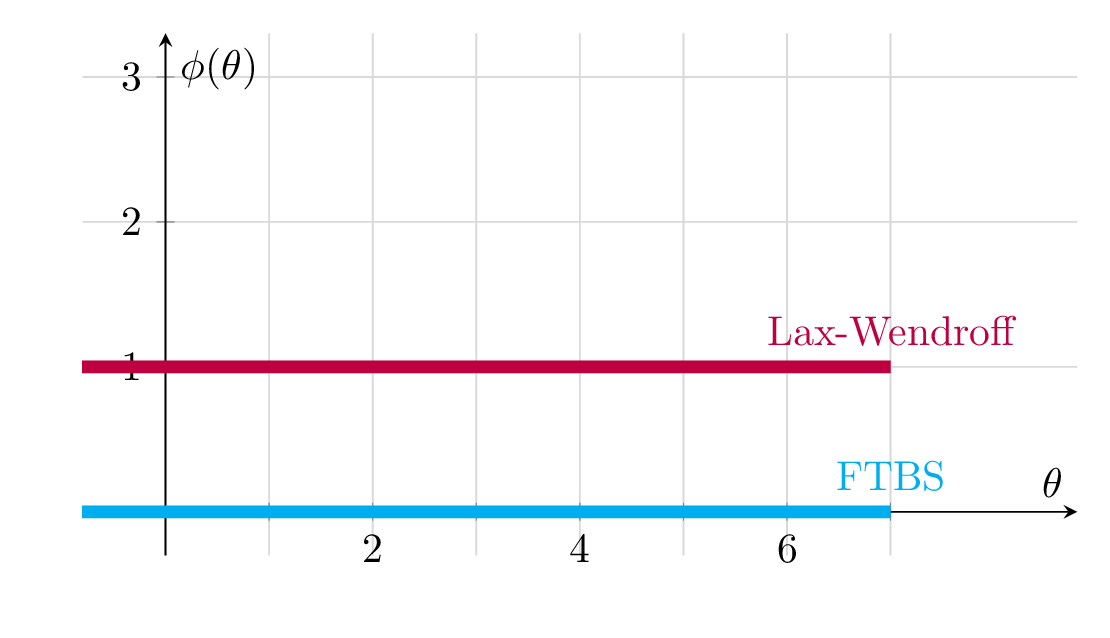
Fig. 9.3 \(\theta\)-\(\phi\) space for visualizing flux limiters. Two simple flux limiters,\(\phi\equiv0\) (blue) and \(\phi\equiv1\) (red) are sketched. These corresond with the FTBS and the Lax-Wendroff scheme. You can confirm this by inserting the fluxes into the Godunov equation on flux form, and massage the mathematical expression.