5.1. Staggered grids

When you design a grid for a numerical model, it may be useful to think aboiut your grids as boxes, as shown in Fig. 5.1. If your grid is 1D, you will have a row of boxes, if you have a 2D grid, you will have a layer of boxes, and for a 3D grid you will have stacked layers of boxes.

If you are dealing with more than one variables, you need to think about where the grid points for each variable should be located within the boxes. The easiest option is to co-locate all the grid points in the center of each box, as illustrated in Fig. 5.1. This is called a non-staggered grid. In the illustration, you see the variables pressure, p and velocity, u positioned in the box centers. Choosing this option makes the coding more care-free, but it turns out that this is not the most suitable placements for these variables.

Think about the physics governing pressure and velocity. Imagine you have a box of water at time step t=0, where water is leaving on the right side faster than it is filling from the left side. This means that you are reducing the amount of water in your box, and the pressure should naturally decrease. If you think of this in terms of the shallow water equation (Eq. (2.17)), where pressure is replaced by sea surface elevation, this would mean that the surface elevation sinks. However, this physical interpretation relies on our knowledge that the velocity at the two box interfaces are different. If we co-locate pressure and velocity in the box centers, we do not immediately know if the pressure will increase or decrease. Instead we must make some averaging and calculate the pressure at the next time step, and this procedure may alter the precision of our model.

Therefore, a more meaningful placing of the grid points, is to stagger the grids, i.e., to place the pressure grid points in the box centers, and the velocity grid points along the box walls/interfaces, as illustrated in Figure Fig. 5.1.

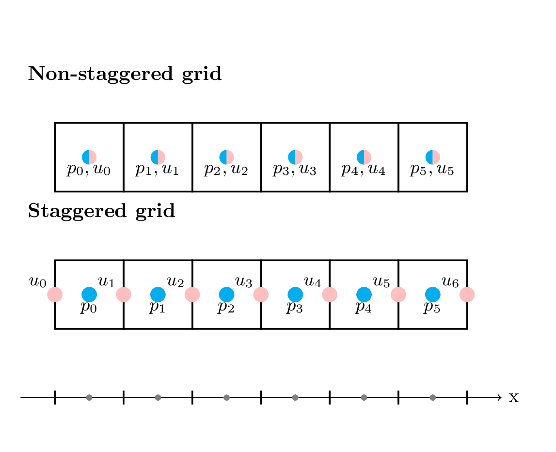
Fig. 5.2 Placement of grid points for multiple variables in co-located/non-staggered grids (top) and staggered grids (bottom). For the staggered grids, the grid points for velocity, u is located at the box walls, while the grid points for pressure, p, is located at the box center.

5.1.1. Staggering reduces effective grid size

Let’s look at the shallow-water gravity waves ((2.21)), but turn it into a 1D case where we ignore advection:

(5.1)\[\begin{split}\begin{aligned} \frac{\partial \eta}{\partial t}&=-H\frac{\partial u}{\partial x}\\ \frac{\partial u}{\partial t}&=-g\frac{\partial \eta}{\partial x}\\ \end{aligned}\end{split}\]

If we concentrate on the first eqution’s spatial derivative, it would be a natural choice to use a centered scheme, taking into account changes in velocity on either side of the grid point. Without staggering, the centered scheme gives \(\frac{\partial u_m}{\partial x}\sim\frac{u_{m+1}-u_{m-1}}{2\Delta x}\). We divide by \(2\Delta x\) and the effective grid size is therefore 2 times the grid resolution. However, if we use staggering, the grid points for \(u\) are only half a grid cell away from the grid point for \(\eta\). The centered scheme now becomes \(\frac{\partial u_m}{\partial x}\sim\frac{u_{m+1/2}-u_{m-1/2}}{\Delta x}\) and the effective grid size is the same a the grid resolution.

Note

The indexing of the grids may easily become confusing. If you look at it from the perspective of \(\eta\) having grid points in the center of the cells, with indexes \(...,m-2,m-1,m,m+1,m+2,...\) the grid points for \(u\) will be located at the indexes \(..., m-5/2,m-3/2,m-1/2,m+1/2,m+3/2,m+5/2,...\). However, this way of looking at it becomes hard to translate into code. Instead, you can think of it as different grids for \(\eta\) and \(u\). it would be clean to use differnet letters for the indexes for \(\eta\) and \(u\), but this becomes messy when you have many coupled equations and variables. Therefore, the common practice is to use the same index names (\(m-1, m-, m+1\)) but define the grid for velocity, \(u\), to be leading or lagging a half grid cell with respect to the \(\eta\)-grid.

Note

When you design your staggered grids, consider how many grid points you need for each variable. In the example above, it makes sense to have one more grid point for \(u\) than for \(\eta\) so that each \(\eta\)-point at the center of a grid cell has information of the velocity, \(u\) on both the grid cell interface to the left and right. In python, where indexes start at zero, it would be useful to let \(u\) lead with respect to \(\eta\), so that \(u_0\) is half a grid cell before \(\eta_0\). This way, the indexes of your arrays will be easier to keep trak of. Another bonus with organizing the grid this way, is that you no longer need boundary conditions for \(\eta\). You only need boundary conditions for \(u\).

5.1.2. Staggering in time - a worked example with inertial oscillatons

If we solve coupled equations, we can use staggering in time to improve our solution. The principle is the sam as for staggering in space, where we use solutions at different time instances for different variables. Inertial oscillations are a great example for demonstrating how this works.

The coupled equations for inertial oscillations described in Section 2.4 and (2.8) are:

\[\begin{split}\begin{aligned} \frac{\partial u}{\partial t}-fv&=0&\quad (i)\\ \frac{\partial v}{\partial t}+fu&=0&\quad (ii) \end{aligned} \end{split}\]

The equations are coupled, meaning that the variables \(u\) and \(v\) appear in both equations, and you can not solve one equation without simultaneously solving the other. We can solve these equations using a simple forward in time scheme without any form of staggering:

(5.2)\[\begin{aligned} u_m^{n+1}&=u_m^n-\frac{f}{\Delta t}v_m^n v_m^{n+1}&=v_m^n+\frac{f}{\Delta t}u_m^n \end{aligned}\]

Figure fig:InertialOsc illustrate the scheme. Since there are no space derivatives in these equaitons, we do not need to invoke neighboring points of \(u_m\) or \(v_n\) in the illustrations.

XXX Insert illustration of schemes XXX

If we now try to stagger in time, we can first solve the equation for \(u\), and then use the new estimate \(u_m^{n+1}\) to solve the eqution for \(v\), resulting in the time-staggered scheme of (5.3):

(5.3)\[\begin{aligned} u_m^{n+1}&=u_m^n-\frac{f}{\Delta t}v_m^n v_m^{n+1}&=v_m^n+\frac{f}{\Delta t}u_m^{n+1} \end{aligned}\]

In the code cell below, you can see the result of the two different solution schemes ((5.2) and (5.3)).

XXX Insert puthon code to show the results of the two different schemes and the analytical solution XXX

5.1.3. Staggering in both time and space

For coupled equations with derivatives in both time and space, you can stagger the numerical schemes in both time and space. Here, we will look into the 1D shallow-water gravity waves without advection ((5.1)) to learn why this is a wise thing to do.

In the following, we use a grid staggering in time, where the grid index for \(u\) is leading the index for \(\eta\). This means, for example, that \(u_m\) i located half a grid cell to the left of \(\eta_m\).

The unstaggered solution

The centered in time, centered in soace (CTCS) scheme for the unstaggered solution, becomes:

(5.4)\[\begin{aligned} \frac{\eta_m^{n+1}-\eta_m^{n-1}}{2\Delta t}&=-H\frac{u_{m+1}^n-u_{m-1}^n}{2\Delta x} \frac{u_m^{n+1}-\u_m^{n-1}}{2\Delta t}&=-g\frac{\eta_{m+1}^n-\eta_{m-1}^n}{2\Delta x} \end{aligned}\]

We can now derive a single equation for \(\eta\) by taking \(\frac{\partial}{\partial t}\) of the first equation and \(\frac{\partial}{\partial x}\) of the second equation using a centered numerical scheme. Then we can combine the equations to eliminate \(u\). Note that when we do this exercise numerically, we must differentiate each instance of \(u\) and \(\eta\) with the chosen scheme. The first term of the first equation,\(\eta_m^{n+1}\), when differentiated with respect to time in a central scheme becomes \(\frac{\eta_m^{n+2}-\eta_m^n}{2\Delta t}\). After differentiation we are left with:

\[\begin{split}\begin{aligned} \left(\frac{\eta_m^{n+2}-\eta_m^n}{2\Delta t}-\frac{\eta_m^{n}-\eta_m^{-2}}{2\Delta t}\right)\frac{1}{2\Delta t}&=-\frac{H}{2\Delta x}\left(\frac{u_{m+1}^{n+1}-u_{m+1}^{n-1}}{2\Delta t}-\frac{u_{m-1}^{n+1}-u_{m-1}^{n-1}}{2\Delta t} \right)\\ \left(\frac{u_{m+1}^{n+1}-u_{m-1}^{n+1}}{2\Delta x}-\frac{u_{m+1}^{n-1}-u_{m-1}^{n-1}}{2\Delta x}\right)\frac{1}{2\Delta t}&=-\frac{g}{2\Delta x}\left(\frac{\eta_{m+2}^{n}-\eta_{m}^{n}}{2\Delta x}-\frac{\eta_{m}^{n}-\eta_{m-2}^{n}}{2\Delta x} \right) \end{aligned}\end{split}\]

Here, you can see that the terms for \(u\) appears in bth equation. By inserting the value for \(u\) from the second equation into the first and rearranging, we get:

\[\eta_m^{n+2}-2\eta_m^n+\{n-2}=\frac{gH\Delta t^2}{\Delta x^2}(\eta_{m+2}^n-2\eta_m^n+\eta_{m-2}^n)\]

This scheme look very much like the solution to the classical wave equTION. However, the schem has only even numbered indexes \(m\) and \(n\). This means that there is no connection between neighboring grid points in time or space. Two solutions can exist simultaneously (one for odd indexes and one for even indexes, or more precisely four solutions if you consider odd spatial indexes existing with either odd or even time indexes and the same for even number space indexes.) This is extremely problematic in a numerical scheme, since the different solutions may end up very different over time. This problem is also referred to as a checkerboard problem, since you can color the grid cells according to which solution they belong to, giving you a checkerboard pattern.

The staggered solution

For the staggered solution, we choose an FTCS scheme. Here you need to consider the notation of the indexes. It is useful to make a little sketch to help you remember where the grid points are relative to each other. Here, we will write up both variations, so that you can check how this looks. First, we write up the scheme using the exact grid point location, where the \(u\)-grid is placed on the half grid points.

\[\begin{split}\begin{aligned} \frac{\eta_m^{n+1}-\eta_m^n}{\Delta t}&=-\frac{H}{\Delta x}\left(u_{m+1/2}^n-u_{m-1/2}^n \right)\\ \frac{u_{m+1/2}^{n+1}-u_{m-1/2}^n}{\Delta t}&=-\frac{g}{\Delta x}\left(\eta_{m+1}^{n+1}-\eta_m^{n+1} \right) \end{aligned}\end{split}\]

If we choose to let \(\eta_m\) be located half a grid point to the left of \(u_m\), a centered scheme in space will look like a forward scheme in the equation.

\[\begin{split}\begin{aligned} \frac{\eta_m^{n+1}-\eta_m^n}{\Delta t}&=-\frac{H}{\Delta x}\left(u_{m+1}^n-u_m^n \right)\\ \frac{u_m^{n+1}-u_m^n}{\Delta t}$=-\frac{g}{\Delta x}\left(\eta_{m+1}^{n+1}-\eta_m^{n+1} \right) \end{aligned}\end{split}\]

Next, we do the same procedure as for the unstaggered grid. We differentiate the first equation with respect to time, and the second equation with respect to space. Then we combine the equations to derive a single equation for \(\eta\):

\( (\eta_m^{n+1}-2\eta_m^n+\eta_m^{n-1})=-\frac{gH\Delta t^2}{\Delta x^2}(u_{m+1}^n-2u_m^2+u_{m-1}^n) \)

This is exactly the same scheme as we get if we solve the classical wave eqution using a CTCS scheme ((11.5)). Here, the scheme includes both odd and even indexes in space and time, and we get one single numerical solution incorporating all the grid points. This makes the staggered solution a much better choice thand the unstaggered scheme for solving the 1D shallow-water gravity waves.

5.1.4. Arakawa grids in 2D

In 2D, there are more options for placement of grid points. If we make a 2D extension of the staggered grid above - and also an extension of the physics, we get a grid as illustrated in Fig. 5.3. This is called an Arakawa C-grid. Arakawa and Lamb published a paper in 1977 (Arakawa and Lamb [AL77]), describing 5 different grid point configurations. These are commonly referred to as Arakawa grids, and includes:

• Arakawa-A: The non-staggered grid, where all variables are defined in the same points

• Arakawa-B: The pressure and other scalars are defined in the box center, and velocity, u and v, are located in the box corners

• Arakawa-C: The pressure and other scalars are defined in the box center, the eastward velocity, u is defined along east/west box walls, and the northward velocity, v, is defined along north/south box walls, as depicted in Fig. 5.3

• Arakawa-D: The same as Arakawa-D, but rotated 90 degrees, so that u and v swap places

• Arakawa-E: The box is rotated 45 degrees, so that u and v can be co-located in the corners

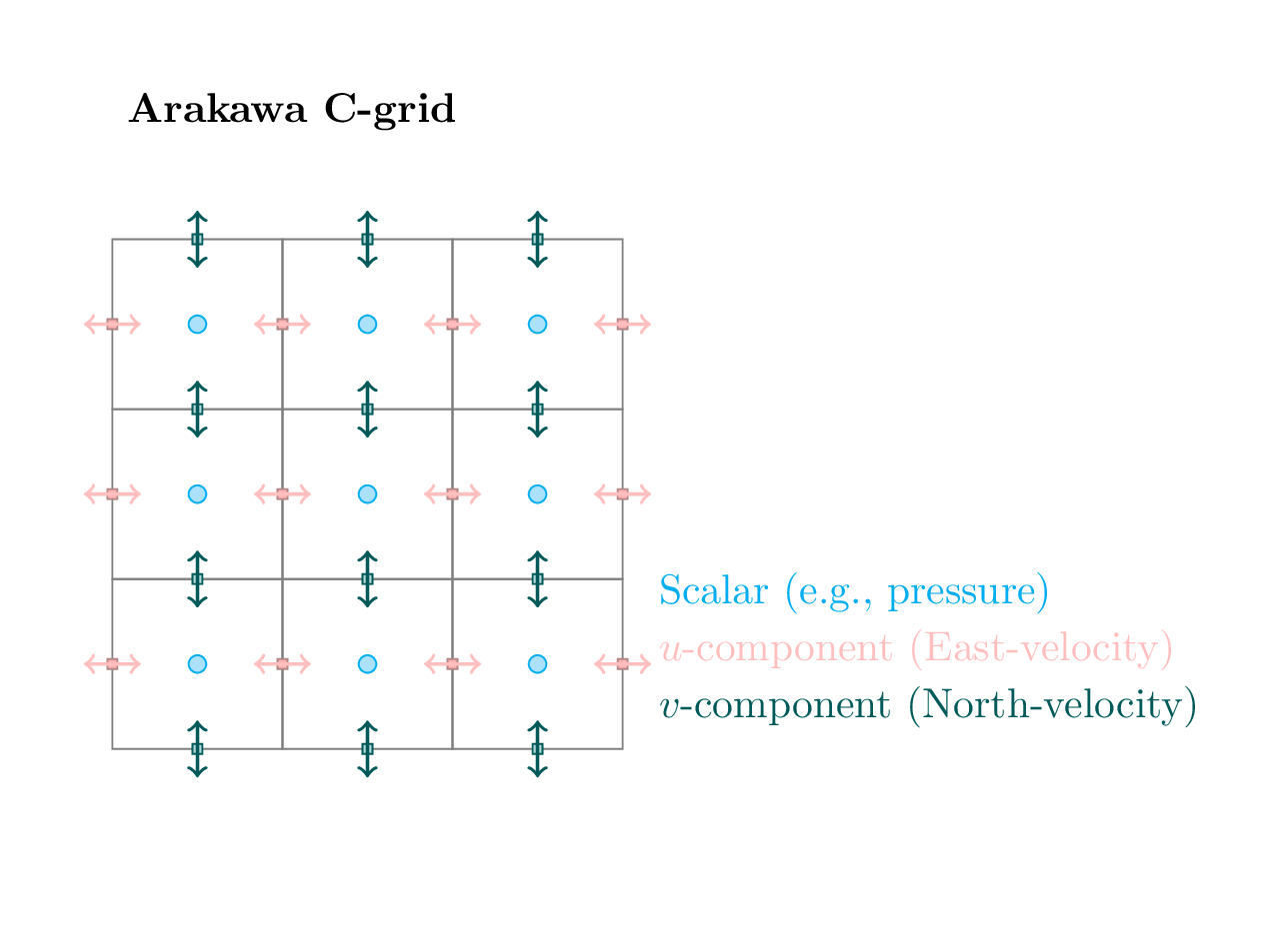
Fig. 5.3 The Arakawa-C grid for 2 dimensions. Pressure and scalar variables are located in the grid centers. The velocity grid points for the eastern direction, u, are located on the east/west box boundaries, while the velocity grid cells for the northern direction, v, are located along the north/south boundaries.

The Arakawa-C grid is one of the most common configurations in geophysical fluid modelling. However, som models use Arakawa-B grids or other configurations. Familiarize yourself with a model’s grid, either you will design the model, run model experiences on a common model, or analyze data from model outputs.

5.1.5. Staggered grids in 3D

Most 3D models using staggered grids consider extends the physical idea of the 2D grids to 3D. If you are using an Arakawa-C grid, you would, for example place the vertical velocity at the floor/roof of each grid box.

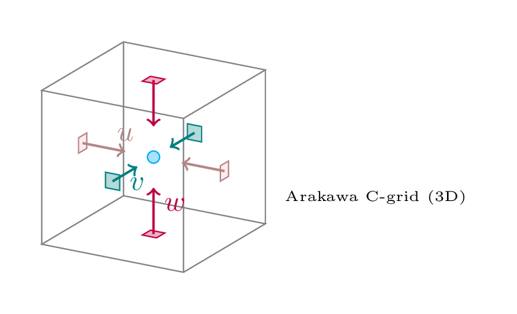
Fig. 5.4 The Arakawa-C grid for 3 dimensions. Pressure and scalar variables are located in the grid centers. The velocity grid points for the eastern direction, u, are located on the east/west box boundaries, while the velocity grid cells for the northern direction, v, are located along the north/south boundaries, and the grid cells for the vertical velocity, w, are located on the floor/roof of the box.