2.4. Inertial oscillations

Inertial oscillations is a special phenomenon occuring when Earth´s rotation (coriolis) is the only force that cause local acceleration

Starting with the 2D Navier Stokes equation (2.4) and removing all terms except local acellaration and coriolis, we are left with:

definition:InertialOscillations)=

Inertial Oscillations

(2.8)\[\begin{split}\begin{aligned} \frac{\partial u}{\partial t}-fv&=0&\quad (i)\\ \frac{\partial v}{\partial t}+fu&=0&\quad (ii) \end{aligned} \end{split}\]

Note

Equation (2.8) is an example of coupled differential equations. When we use the term ‘coupled’, we mean that the two equations are connected, with one or more parameters appearing in both equations. Here, you can see that the first equation, which is an expression for \(\frac{\partial u)(\partial t)\), contains the variable \(v\), and vice versa. We must therefore solve these equations together, since we cannot solve first one an then the other. This is true both for the analytical and the numerical solution. However, for the analytical solution, we may solve them sequentially for each time step.

We can combine these equations, by expressing the as \(U=u+iv \quad(iii)\). By differentiating \((iii)\) with respect to time, and inserting the expressions from \((i)\) and \((ii)\), we get:

(2.9)\[\frac{\partial U}{\partial t}=-ifU\]

This is a classical first order Ordinary Differential Equation (ODE) with the solution:

(2.10)\[U=Ae^{ift} = A(cos(ft)-isin(ft))\]

If we assume an initial condition on the form \(U(t=0)U_0=u_0+iv_0\), this gives us \(U_0=A(cos(0)-isin(0))=A(1-0)=A\). We can now write out the full solution as:

(2.11)\[U=U_0e^{ift} = U_0(cos(ft)-isin(ft))\]

Try it!: Try for yourself to set \(U_0=i\) and find the \(u\) and \(v\) at timesteps \(0, \frac{\pi}{4f}, \frac{\pi}{2f}, \frac{3\pi}{4f}, \frac{\pi}{f}\). Does these values match the sketch below?

The inertial oscillations do not move in space like the advection or diffusion equations did (we have no \(\partial/\partial x\)-terms). The solutions provide a change of current/wind direction with time only. The solution will be a circular movement that is stationary with time (see Figure Illustration of the velocity vectors for the inertial oscillation at various times steps. Herre, the initial condition is set to U_0=iv. The velocity vectors rotate clockwise with time.).

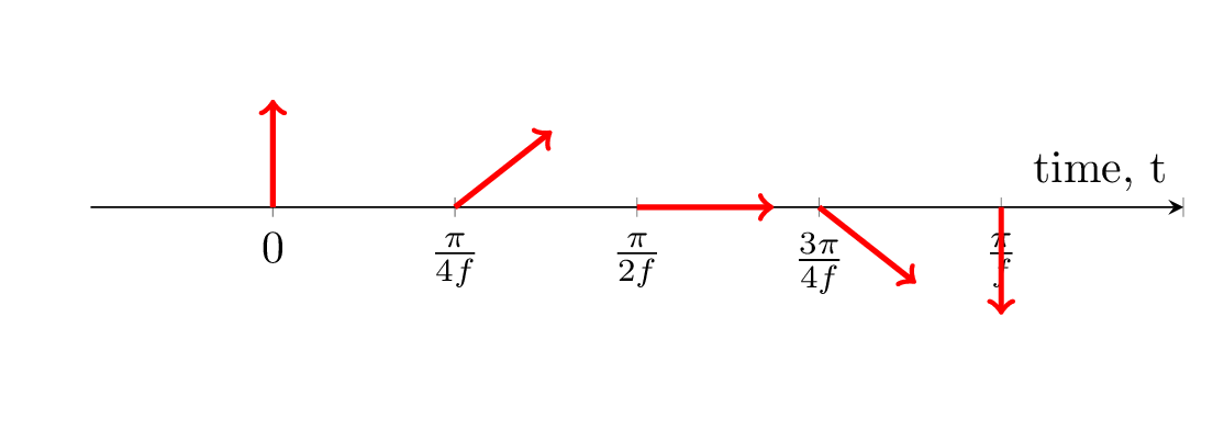
Fig. 2.1 Illustration of the velocity vectors for the inertial oscillation at various times steps. Herre, the initial condition is set to \(U_0=iv\). The velocity vectors rotate clockwise with time.

In real life, there is seldom/never a pure inertial balance, and the inertial oscillations will be advected by the background current as depicted in Figure Drifter tracks from an October storm in 1987, deployed during the Ocean Storms Experiment campaign in the northeast Pacific. Image from vanMeurs1998.. These inertial oscillations were observed during a drifter campaign in the northeast Pacific furing an October storm.

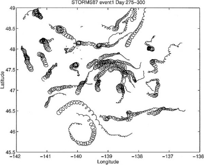
Fig. 2.2 Drifter tracks from an October storm in 1987, deployed during the Ocean Storms Experiment campaign in the northeast Pacific. Image from Van Meurs [VM98].