9.1. Godunov’s method

This chapter is co-written with Sigrid Christine Pedersen (student in GEOF211 spring 2025)

The Godunov scheme is a numerical method that aligns with the conservation laws for hyperbolic partial differential equations. It computes the solution at the next time step through the following three-step process:

1. Compute cell-averaged values and reconstruct a polynomial approximation, \(\tilde{q}_x^t\), for the solution \(q_x^t\) within each grid cell.

2. Use the reconstructed solution as the initial condition to integrate the advection equation over the next time step.

3. Compute the new cell-averaged values at the updated time level \(t^{n+1}\).

9.1.1. Godunov Step 1

The simplest type of polynomial reconstruction is a linear expression such as:

(9.1)\[\tilde{q}_k^t(x,t^n)=q_k^n+(x-x_k)\sigma_k^n,\]

where \(\sigma_k^n=\frac{{\partial q}}{\partial x}\rvert_k^n\) is the slope of the reconstructed linear \(\tilde{q}\). Note that the full reconstructed signal is made up of many linear segments - one segment per grid cell. The reconstructed signal is, therefore, not a continuous function. Fig. 9.1 shows an example of a reconstructed signal, \(\tilde{q}\), consisting of linear segments (purple lines). The segments extend over one grid cell each, and passes through the functional values \(q_k^n\), but are not connected at the grid cell edges.

We can decide how we want to express this slope numerically. We could, for example, use a:

• Forward scheme, also called a downwind slope: \(\sigma_k^n = \frac{q_{k+1}^n - q_k^n}{\Delta x}\)

• Backward scheme, also called an upwind slope: \(\sigma_k^n = \frac{q_k^n - q_{k-1}^n}{\Delta x}\)

• Centered scheme:\(\sigma_k^n = \frac{q_{k+1}^n - q_{k-1}^n}{2 \Delta x}\)

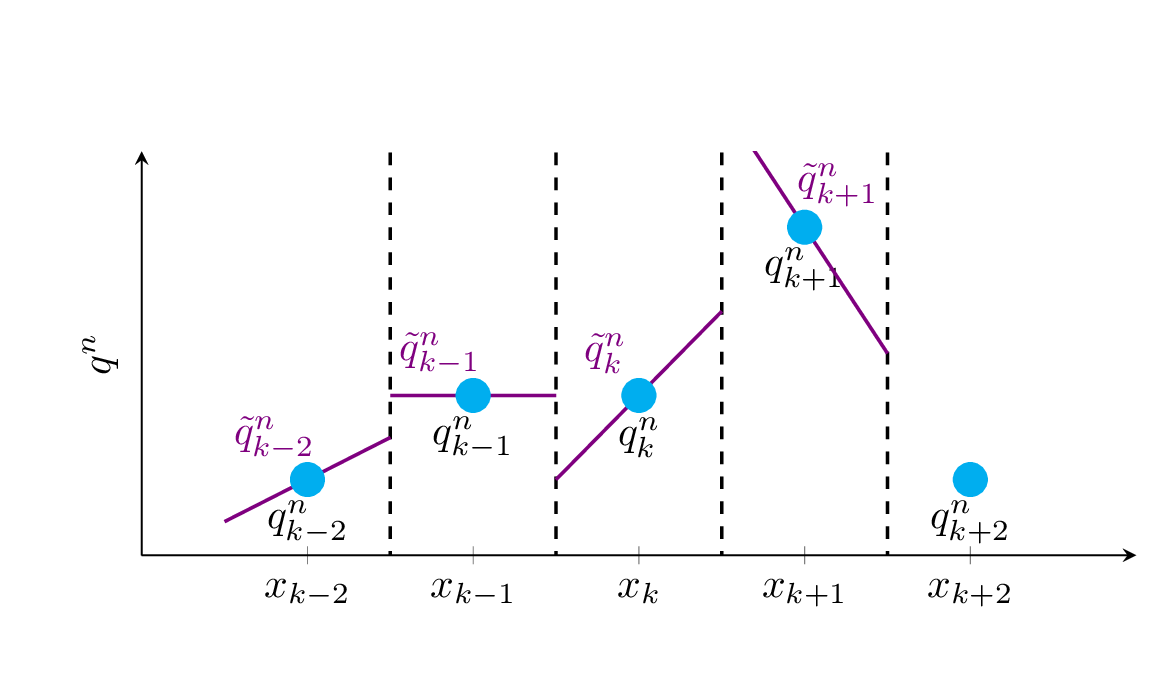
Fig. 9.1 Illustration of a linear reconstruction \(\tilde{q}\) (purple line segments) for a set of functional values \(q\) (blue markers). The reconstruction is based on the downwind slope (forward differencing). If you, for example, extend the purple line segment at grid cell \(k\) on the right hand side, you will notice that it pass through the functional value of the grid cell to the right - i.e., a forward differencing.

Fig. 9.1 shows an example of an upwind slope, using a forward differencing for \(\sigma_k^n\).

Note

You can use a ruler to practice finding the reconstructed signal on a piece of paper. Sketch two axes and some functional values, \(q_k^n\). To find the reconstructed signal for the downwind slop (Forward scheme), you can place the ruler so it touches the functional values \(q_{k+1}^n\) and \(q_k^n\). Then you draw a line that covers the grid cell \(k\), from the left border at \(k-1/2\) to the right cell border at \(k+1/2\). If you want to find the upwind slope, you must repeat the exercise by placing the ruler through \(q_{k-1}^n\) and \(q_k^n\). If you make the exercise for the centered scheme, you must first find the slope by placing the ruler from \(q_{k-1}^n\) to \(q_{k+1}^n\) and then sliding the ruler vertically until it passes through your point \(q_k^n\).

9.1.2. Godunov Step 2

The first part of step 2, is to advect the reconstructed signal using the characteristics \(x-at\), and track inflow and outflow of cell \(q_k^n\).

Fig. 9.2 illustrates how this will look in terms of grid cells. Let’s say we look at an advection equation where \(a>0\), so that the signal is moving towards the right. Flow will then enter the grid cell at the left border \(k-1/2\) and exit at the right border at \(k+1/2\).

We use the charachteristics of the advection equation \(x-at\), since the solution of the advection equation lies along these charachteristics. The charactheristcs are linear, with a slope \(a\), seen in Fig. 9.2.

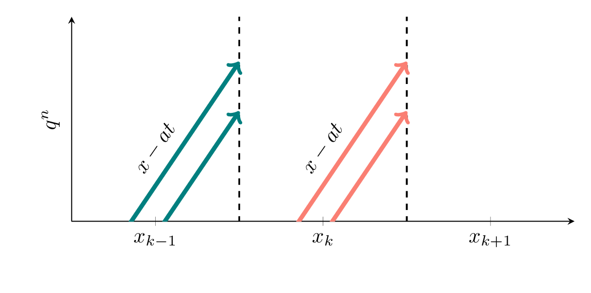
Fig. 9.2 Illustration of a the characteristics of the linear advection equation \(x-at\). For grid cell \(k\)m there is an infow from the \(k-1\) cell at cell border location \(k-1/2\) (\(\color{teal}{\text{teal color}}\)) and outflow from the \(k\) grid cell at \(k+1/2\) (\(\color{salmon}{\text{salmon color}}\)).

Outflow: For the flow out of the box at \(k+1/2\), we insert \(\color{salmon}{x=x_{k+1/2}-a(t-t^n)}\) into equation (9.1) from step 1. Note that for the outflow, the \(k\)-cell is the mother cell of the flow. We can therefore keep all the \(k\)’s in equation (9.1) as they appear.

(9.2)\[\begin{split}\begin{aligned} \tilde{q}_k^n(x,t^n)&=q_k^n+({\color{salmon}{x_{k+1/2}-a(t-t^n)}}-x_k)\sigma_k^n\\ &=q_k^n+(\frac{\Delta x}{2}-a(t-t^n))\sigma_k^n \end{aligned}\end{split}\]

Inflow: For the flow into the box at \(k-1/2\), we insert \(\color{teal}{x=x_{k-1/2}-a(t-t^n)}\) into equation (9.1) from step 1. Note that for the inflow, the \((k-1)\) cell is the mother cell of the flow. We must, therefore, replace all the instances of \(k\) in equation (9.1) with \(k-1\).

(9.3)\[\begin{aligned} \tilde{q}_{k-1}^n(x,t^n)&=q_{k-1}^n+({\color{teal}{x_{k-1/2}-a(t-t^n)}}-x_{k-1})\sigma_{k-1}^n &=q_{k-1}^n+(\frac{\Delta x}{2}-a(t-t^n))\sigma_{k-1}^n \end{aligned}\]

With the inflow and outflow defined, we can integrate the reconstructed signal over one time step. This will provide us with the net flow through a grid cell.

(9.4)\[\begin{split}\begin{aligned} \int_{t^n}^{t^{n+1}}\frac{\partial q}{\partial t}\,dt&=-\int_{t^n}^{t^{n+1}}a\frac{\partial q}{\partial x}&=-\int_{t^n}^{t^{n+1}}\frac{\text{outflow-inflow}}{\Delta x}\,dt\\ q_k^{n+1}-q_k^n&=-\int_{t^n}^{t^{n+1}}a\frac{\partial \tilde{q}}{\partial x}&=-a\int_{t^n}^{t^{n+1}}\frac{\tilde{q}_k^n-\tilde{q}_{k-1}^n}{\Delta x}\,dt\\ \end{aligned}\end{split}\]

We finally substitute \(\tilde{q}_{k-1}^n\) and \(\tilde{q}_{k}^n\) into (9.4) and achieve the general Godunov scheme:

(9.5)\[q_k^{n+1} = q_k^n - a \frac{\Delta t}{\Delta x} \left( q_k^n - q_{k-1}^n \right) - \frac{a \Delta t}{2} \left( 1 - \frac{a \Delta t}{\Delta x} \right) \left( \sigma_k^n - \sigma_{k-1}^n \right)\]

9.1.3. Godunov Step 3

The final step, is to choose which scheme you want to use for the slope \(\sigma_k^n\) determines the specific variant of the scheme.

• The downwind slope, \(\sigma_k^n = \frac{q_{k+1}^n - q_k^n}{\Delta x}\) gives you the Lax-Wendroff

• The upwind slope, \(\sigma_k^n = \frac{q_{k}^n - q_{k-1}^n}{\Delta x}\) gives you the Beam-Warming scheme

• The centered slope, \(\sigma_k^n = \frac{q_{k+1}^n - q_{k-1}^n}{2\Delta x}\) gives you the Fromm scheme

The three schemes are second-order accurate, offering improved precision compared to first-order methods such as FTBS and Lax-Friedrichs. As a result, Godunov’s schemes are generally expected to yield better performance.

To improve the solution further, overshoots and undershoots need to be addressed. These typically arise when the upwind and downwind slopes have opposite signs. A minmod limiter is used to prevent such non-physical oscillations. It does this by selecting the slope with the smallest variation at each time step.

The Godunov method is not only applicable to the advection equation. However, you must adapt the charachteristics in step 2 to the equation you are considering.

Note

Although it may be tempting to insert the choice of \(\sigma_k^n\) into Equation (9.5) the one-step solution before coding, it will be useful to calculate the slope \((\sigma_k^n-\sigma_{k-1}^n)\) separately. We will learn how to make wise choices based on slope characteristics, and keeping these calculations tidy will be essential!

9.1.4. Min-mod limiters

If we study the upwind and downwind slopes in an area close to grid cell \(k\), we can make som intentional choices of which slope to use where. A steep slope indicates a strong gradient, while a mild slope indicates a weak gradient. It is often benefitial to choose the mildest of the two slopes.

In places where the signal undulates (i.e., going up and down), the upwind and downwind slopes will have opposite signs. Here, we risk getting overshoots and undershoots from our Godunov approach. To reduce this problem, we can define a minmod limiter. You can regard a limiter as a rule for what slope, \(\sigma_k^n\) to choose at a given grid cell.

(9.6)\[\sigma_k^n=\text{minmod} \left (\frac{q_k^n-q_{k-1}^n}{\Delta x},\frac{q_{k+1}^n-q_{k}^n}{\Delta x}\right)\]

, where minmod is defined as:

(9.7)\[\begin{split}\text{minmod}(a,b)\begin{cases} a\,\, \text{if } |a|&<|b|\,\text{and } ab > 0 \\ b\,\, \text{if } |a|&>|b|\,\text{and } ab > 0 \\ 0\,\, \text{if } ab& \leq 0 \end{cases}\end{split}\]