1.6. Fourier transforms

1.6.1. Superposition of waves

When two or more waves meet, for example when two boats pass each other, their wake waves will overlap in space. The surface displacement (amplitude) will, at any point, be the sum of the surface displacement for the individual waves.

When looking at the ocean surface, the surface elevation can be regarded as the sum of (superposition) of many waves of different frequencies and phases.

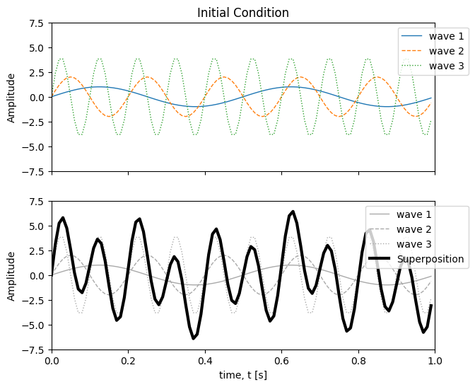
In the figure, you can see three individual sine waves with varying frequencies and amplitudes. The first wave (blue) has 2 oscillations per seconds, the second wave (orange) has 5 oscillations per second, and the third wave (green) has 10 oscillations per second. The black, bold line shows the superposition of the three waves. The amplitude at any point in time, is the sum of the amplitudes of the three individal waves.

Show code cell source

Hide code cell source

import numpy as np
import matplotlib.pyplot as plt

# Create time values
Fs=100 # sampling rate -. number of samples per second
t = np.arange(0,1,1/Fs) #one cycle

#define frequencies, phases, and amplitudes of three sine waves
frequencies=np.array([2.,5.,10])
amplitudes=np.array([1.,2.,4.])

# compute the wave signals
wave1 = amplitudes[0] * np.sin(2 * np.pi * frequencies[0] * t)
wave2 = amplitudes[1] * np.sin(2 * np.pi * frequencies[1] * t)
wave3 = amplitudes[2] * np.sin(2 * np.pi * frequencies[2] * t)

# Add the sine waves together
superposition_wave = wave1 + wave2 + wave3

#plot the wave signals
fig, ax = plt.subplots(2, 1, figsize=(7, 6), sharex=True)
ax[0].set_xlim(( 0, 1))
ax[0].set_ylim((-7.5, 7.5))

line1, = ax[0].plot(t, wave1,'-', lw = 1, label='wave 1')
line2, = ax[0].plot(t, wave2,'--', lw = 1, label='wave 2')
line3, = ax[0].plot(t, wave3,':', lw = 1, label='wave 3')

ax[1].plot(t, wave1,'-',color='darkgrey', lw = 1, label='wave 1')
ax[1].plot(t, wave2,'--',color='darkgrey', lw = 1, label='wave 2')
ax[1].plot(t, wave3,':',color='darkgrey',lw = 1, label='wave 3')
line4, = ax[1].plot(t, superposition_wave,'k', lw = 3, label='Superposition')

ax[0].set_ylabel('Amplitude')
ax[0].set_title("Initial Condition")
ax[0].legend(loc="upper right", bbox_to_anchor=(1.1, 1))
ax[1].legend(loc="upper right", bbox_to_anchor=(1.1, 1))
ax[1].set_ylabel('Amplitude')
ax[1].set_xlabel('time, t [s]')
ax[1].set_ylim((-7.5, 7.5))

(-7.5, 7.5)

1.6.2. Time/space domain versus frequency domain - The Fourier Series

A data signal can be represented in either a time/space domain or a frequency domain.

The time domain represents how the signal (for example air temperature) is changing with time, \(t\). The time is running along the horizontal axis and the temperature is in the vertical axis. Mathematically, we would say that the temperature is a function of time, \(y(t)\). Similarly, the space domain represents how the signal (for example air temperature) is changing with space or distance, \(x\). Then, the resulting function would be \(y(x)\).

To get a meaningful interpretation of the frequency domain, we must first approximate our signal by the sum of the mean value of our signal, \(\bar{y(t)}\), and a superposition of many waves with different frequencies, amplitudes, and phases, \(T\). The more frequencies, \(\omega_n\) with unit [radians per time], we include in the superposition, the better the approximation is. The approximation is typoically valid within a certain time period, \(T\). The frequencies are related to the time period, through \(\omega_n=2\pi/T\).

(1.31)\[y(t)=\bar{y(t)}+\sum_n[A_ncos(\omega_n t)+B_nsin(\omega_n t)]\]

The number of frequencies we can reolve in a time series, depend on the time interval and the sampling frequency. To resolve a wave signal, we need at least 2 datapoints per wavelength. The highest resolveable frequency, will therefore be \(f_N=(N/2)/N\Delta t=1/2\Delta t\). This is called the Nyquist frequency.

Another way of representing the function \(y(t)\) as a Fourier series, is to note that \(\bar{y(t)}\) can be written as \(A_n/2\):

(1.32)\[y(t)=\frac{A_0}{2}+\sum_n[A_ncos(\omega_n t)+B_nsin(\omega_n t)]\]

The amplitude of each wave in the superposition, can be derived from the following equations:

(1.33)\[\begin{split}A_n=\frac{2}{T}\int_{0}^{T}f(t)cos(\omega_n t)dt, n=0,1,2,...\\ B_n=\frac{2}{T}\int_{0}^{T}f(t)sin(\omega_n t)dt, n=1,2,...\end{split}\]

We can also construct the Fourier series using complex notation for currents, e.g., by stating that \(U(t)=u(t)+iv(t)\), when \(u(t)\) and \(v(t)\) are velocities in east and north direction, respectively:

(1.34)\[U(t)=\sum_{n=0}^\infty c_n e^{i 2\pi\frac{n}{T}t}\]

, where

(1.35)\[c_n=\frac{1}{T}\int_{0}^{T}U(t)e^{-i\frac{2\pi}{T}t}dt\]

1.6.3. The Fourier transform pair

When we have created our approximated signal, we can calculate the amount of energy (wave amplitude) related to each frequency. The result is a function that displays the energy as a function of frequency. If we let \(t\rightarrow \infty\) and include enough wave frequencies to allow \(n/T \rightarrow \xi\) we can now write a function of the amount of energy as in terms of each wave. This is how our signal looks in the frequency domain, and this function is called the Fourier transform. There are two versions, one continuous and one discrete:

For a continuous functions, \(y(t)\) the Fourier transform pair is defined:

(1.36)\[\begin{split}\begin{aligned} Y(f)&=\int_{-\infty}^\infty y(t)e^{-i2\pi ft}dt\\ y(t)&=\int_{-\infty}^\infty Y(f)e^{i2\pi ft}df\\ &=\frac{1}{2\pi}\int_{-\infty}^\infty Y(f)e^{i\omega t}d\omega \end{aligned}\end{split}\]

,where \(\omega=2\pi f\). The functions are inverse set of functions.

For discrete data series (in time or space), the Fourier transform is:

(1.37)\[Y(f)=\Delta t \sum_{-\infty}^\infty y_n e^{-i2\pi ft}\]

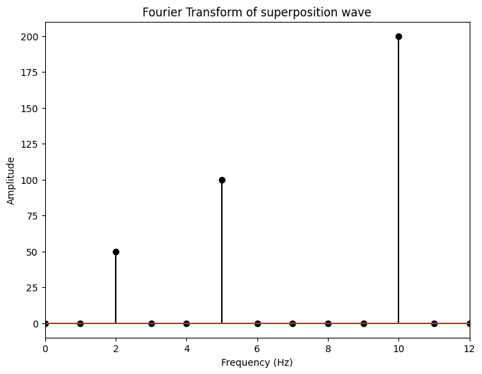
Here, the function \(Y(f)\) represent energy as a function of the frequency \(f\). If the signal consisted of just one pure sine wave, the graph of \(Y(f)\) would contain a single spike at the frequency of this sine wave. For the superposition of the three waves in the example above, we get one spike for each of the frequencies 2, 5, and 10 cycles per second.

Show code cell source

Hide code cell source

#import fft package using only real numbers into the transform
from scipy.fft import rfft, rfftfreq

# Calculate N
N = len(t)

# Compute the Fourier transform
frequency_eval_max = 100 #max number of components
superposition_wave_rfft = rfft(superposition_wave, n=frequency_eval_max)
n = np.shape(superposition_wave_rfft)[0] 
frequencies_rel=rfftfreq(N, 1 / Fs)
#frequencies_rel = n*Fs/frequency_eval_max * np.linspace(0,1,int(n))

# Plot the Fourier transform
plt.figure(figsize=(8, 6))
#plt.plot(frequencies_rel, np.abs(superposition_wave_rfft),'k',lw=2, label="Fourier Transform")
plt.stem(frequencies_rel, np.abs(superposition_wave_rfft),'k')

plt.title('Spectrum')
plt.xlabel('Frequency[Hz]')
plt.ylabel('Amplitude')

plt.xlim([0,12])
plt.xlabel("Frequency (Hz)")
plt.ylabel("Amplitude")
plt.title("Fourier Transform of superposition wave")

Text(0.5, 1.0, 'Fourier Transform of superposition wave')

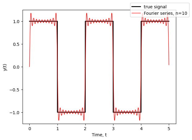
1.6.4. Gibbs phenomenon

In practice, we typically cannot include an infinite number of terms in the Fourier series to represent a signal. using a limited number of components works fine for continuous signals, but will produce errors (overshoots and undershoots) near discontinuities and areas wih strong gradients. This is called the Gibbs phenomenon.

Show code cell source

Hide code cell source

import numpy as np
import matplotlib.pyplot as plt

t = np.arange(0,5,0.001)

# t.astype(int) % 2 will alternate between the value 1 and zero
square_wave = 1 - 2 * (t.astype(int) % 2)

N = 10 #number of frequencies to include
superpos = np.zeros_like(t) #short for superposition

for i in range(N): #loop through the 10 first sine waves
    n = 2*i + 1 #only odd numbers 
    superpos += np.sin(n * np.pi *t) / n #adds the sine wave for n into the superposition so far
superpos *= 4 / np.pi

fig, ax = plt.subplots()
ax.plot(t, square_wave,'k', lw=2,label='true signal')
ax.plot(t, superpos, 'r',lw=1, label='Fourier series, n=10')
ax.legend(loc="center right", bbox_to_anchor=(1.1, 1))
ax.set_ylim(-1.25,1.25)
plt.xlabel("Time, t")
plt.ylabel("y(t)")


plt.show()

1.7. Bonus example code for visualisation of the Fourier components!

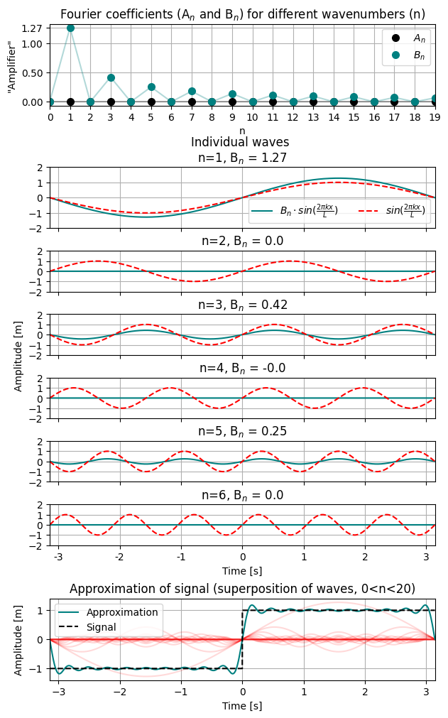
The figure below shows three major parts of the Fourier series:

1. The Fourier components corresponding to how much an individual wave of a given wave number contributes to the signal

2. The individual waves, being the multiple of the individual waves and the Fourier component

3. The superposition of these waves, being simply the sum of each individual wave up to a number N, in this case, taken to be 20 (i.e., 20 Fourier components and 20 individual waves). The example used is of a step function, often used to illustrate Gibbs phenomenon (see above).

The first panel shows the magnitude of each Fourier component (A\(_n\) and B\(_n\)) up to the wavenumber 20 (or 19, counting from 0). Each of the 20 wavenumbers corresponds to waves with different wavelengths (n = 1 corresponds to one waveperiod within the domain, n=2 corresponds to two waveperiods within the domain, and so forth). In the next six panels, the waves corresponding to a wavenumber are shown (n=1 to n=6, red). The same waves are multiplied by the corresponding Fourier component (Teal). We note that all the A\(_n\)-components are zero, so these are not shown. Moreover, every other B\(_n\)-component is zero (seen in the top panel), resulting in no contribution to the superposition. The lowermost panel shows the superposition of the first 20 wavenumbers, which is reduced to include only every other B\(_n\) component.

import numpy as np
import matplotlib.pyplot as plt
from scipy.signal import square
from scipy.integrate import quad
from math import * 

# initialize arrays
x=np.arange(-np.pi,np.pi,0.001) 
y=square(x) 

# number of fourier components to include
n=20
xarr = np.linspace(0,n-1,n) # array for plotting

An=np.zeros([n]) #// defining array
Bn=np.zeros([n])

# Calculate Fourier components
fc=lambda x:square(x)*cos(i*x)  
fs=lambda x:square(x)*sin(i*x)
for i in range(n):
    An[i]=quad(fc,-np.pi,np.pi)[0]*(1.0/np.pi)
    Bn[i] = quad(fs,-np.pi,np.pi)[0]*(1.0/np.pi)

# Make plot
fig = plt.figure(figsize=[7,12])
grid = plt.GridSpec(10,1,height_ratios=[2,0.4,1.5,1,1,1,1,1,0.2,2],hspace=0.5)


# Plot the fourier components
ax = fig.add_subplot(grid[0,0])
ax.set_title('Fourier coefficients (A$_{n}$ and B$_{n}$) for different wavenumbers (n)')
ax.plot(xarr,An,'k',alpha=0.3)
ax.plot(xarr,Bn,'Teal',alpha=0.3)
ax.plot(xarr,An,'o',color='k',markersize=7,label=r'$A_n$')              # Note that all An's are zero, we will therefore neglect them in the next few panels
ax.plot(xarr,Bn,'o',color='Teal',markersize=7,label=r'$B_n$')
ax.legend()
ax.grid()
ax.set(xlim=[0,19],xticks=xarr,ylabel='"Amplifier"',xlabel='n',yticks=[0,0.5,1,np.round(Bn[1],2)])

# Calculate the individual waves (one wave corresponds to one fourier component (=n))
BN = np.zeros([n,x.shape[0]]) 
PN = np.zeros([n,x.shape[0]])
for i in range(1,n):
    BN[i,:] = Bn[i]*np.sin(i*x)     # The wave multiplied by the amplitude of the Fourier component
    PN[i,:] = np.sin(i*x)           # The wave with amplitude: -1 < A < 1

# Plotting the first few waves 
for i in [1,2,3,4,5,6]:#[1,3,5,7,9,11]:
    ax = fig.add_subplot(grid[i+1,0])
    ax.plot(x,BN[i,:],'Teal',label=r'$B_n \cdot sin(\frac{2 \pi k x}{L})$')
    ax.plot(x,PN[i,:],'r--',label=r'$sin(\frac{2 \pi k x}{L})$')
    if i != 1:
        ax.set_title('n='+str(i)+', B$_n$ = '+str(np.round(Bn[i],2)),y=1)
    else:
        ax.set_title('Individual waves \nn='+str(i)+', B$_n$ = '+str(np.round(Bn[i],2)),y=1)
        ax.legend(loc= 'lower right',ncols=2)
    if i == 3:
        ax.set_ylabel('Amplitude [m]',y=0)
    ax.set(ylim=[-2,2],xlim=[-np.pi,np.pi],yticks=[-2,-1,0,1,2],xticks=[-3,-2,-1,0,1,2,3],xticklabels=[])
    ax.grid()
    
ax.xaxis.set_ticklabels([-3,-2,-1,0,1,2,3])
ax.set_xlabel('Time [s]')

# Calculate the sum of the fourier components (i.e., the superposition of the individual waves)
sum=0
for i in range(n):
    if i==0.0:
        sum=sum+An[i]/2
    else:
        sum=sum+(An[i]*np.cos(i*x)+Bn[i]*np.sin(i*x)) # Don't actually need the "An[i]*np.cos(i*x)" part because we know it to be zero for all n.

# plot the actual signal (black), the individual waves/Fourier components (red), and the superposition of the waves (Teal)
ax = fig.add_subplot(grid[9,0])
ax.set_title('Approximation of signal (superposition of waves, 0<n<20)')
for i in range(n):
    ax.plot(x,(An[i]*np.cos(i*x)+Bn[i]*np.sin(i*x)),color='red',alpha=0.15)
ax.plot(x,sum,color='Teal',label='Approximation')
ax.plot(x,y,'k--',label='Signal')
ax.grid()
ax.set(xlabel='Time [s]',ylabel='Amplitude [m]',xlim=[-np.pi,np.pi])
ax.legend()

<matplotlib.legend.Legend at 0x7f8ce7817c40>

You can read more about Fourier series and transforms in Emery and Thompson [ET97].