9.3. Godunov schemes with TVD flux limiters

We know that FTBS has severe dnumerical diffusion, and that Lax-Wendroff can give solutions where oscillations grow near strong gradients. Making a flux limiter that just switch between these two schemes is not necessarily sufficient to provide a good numerical model for the advection equation.

To improve our numerical scheme even further, we can try to ensure that the scheme does not introdue oscillations. Chapter Total Variation (TV) and Total Variation Diminishing (TVD) schemes (part 1) introduced the concept of Total Variation and Total Variation Diminishing (TVD) schemes. We will expand on this concept here, to design improved numerical schemes for advection based on the Godunov approach with flux limiters. This boils down to finding clever values of \(\phi(\theta)\).

We will make a short recap of TVD part 1 from chapter Total Variation (TV) and Total Variation Diminishing (TVD) schemes (part 1). The total variation is a measure of the amount of oscillation in the field:

Definition

(9.16)\[TV(q^n)=\sum_{m=2}^J|(q_m^n-q_{m-1}^n)|\]

A numerical scheme is Total Variation Diminishing if:

Definition

A numerical scheme is total variation diminishing if:

(9.17)\[TV(q^{n+1})\leq TV(q^n)\]

9.3.1. The Godunov scheme on the general form

So - how can we ensure that the Godunov scheme on flux form is TVD?

Do you remember the Harten theorem fro Equation (4.4)?

Consider a general method of the form:

\[q_k^{n+1}=q_k^n-A_{k-1}^n(q_k^n-q_{k-1}^n)+B_k^n(q_{k+1}^n-q_k^n)\]

where the coefficients \(A\) and \(B\) are arbitrary values that may depend on \(q\). (Note that these coefficients are displaced half a grid length to the right, so that, e.g., \(B_k^n\) is valid at \(j+\frac{1}{2}\).) Then it has been shown [Har83] that

Harten’s Theorem

Consider a method on the general form (Equation (4.3)). Then

\[TV(q^{n+1})\leq TV(q^n)\]

if \(A_k^n+B_k^n\leq 1\) and \(A_k^n\geq 0\), \(B_k^n \geq 0\,\, \forall\,k\)

We can now verify that the Godunov scheme with flux limiters for linear advection is TVD. To do so, requires a nit of math. We must first find an expression for the scheme on the general for (Equation (4.3)), and then find restrictions for \(A\) and \(B\).

Step 1: Inserting the fluxes into the equation fo \(q_k^{n+1}\) from Equation (9.15) to find the General form

\[\begin{split}\begin{aligned} q_k^{n+1}& =q_k^n+\frac{\Delta t}{\Delta x}\left[ {\color{salmon}{aq_{k-1}^n}+\frac{a}{2}(1-C)}{\color{teal}{(q_k^n-q_{k-1}^n)\phi(\theta_{k-1/2}^n)}}- {\color{salmon}{aq_k^n}}+\frac{a}{2}(1-C){\color{ForestGreen}{(q_{k+1}^n-q_k^n)\phi(\theta_{k+1/2}^n)}} \right]\\ & =q_k^n- {\color{salmon}{C(q_{k-1}^n-q_{k-1}^n)}} -\frac{C}{2}(1-C)\left[ {\color{ForestGreen}{\phi(\theta_{k+1/2}^n)(q_{k+1}^n-q_k^n)}} - {\color{teal}{\phi(\theta_{k-1/2}^n)(q_k^n-q_{k-1}^n)}} \right] \end{aligned}\end{split}\]

This is not yet on the general form. To get there, we must factorize the scheme in terms of \({\color{violet}{(q_k^n-q_{k-1}^n)}}\). This is not straighforward to guess (it is indeed tempting to leave the term with \((q_{k+1}^n-q_k^n)\) separately), but we will see how it works out:

(9.18)\[q_k^{n+1}=q_k^n-C {\color{violet}{(s_{k-1}^n-q_{k-1}^n)}} -\frac{C}{2}(1-C)\left[ \phi(\theta_{k+1/2}^n)\frac{(q_{k+1}^n-q_k^n)}{{\color{violet}{(q_{k-1}^n-q_{k-1}^n)}}} - \phi(\theta_{k-1/2}^n){\color{violet}{(q_k^n-q_{k-1}^n)}} \right]\]

Noting that the term \(\frac{(q_{k+1}^n-q_k^n)}{{\color{violet}{(q_{k-1}^n-q_{k-1}^n)}}}\) is the same as \({1}/{\theta_{k+1/2}^n}\), we can replace this in equation (9.18), and complete the factorizing of \({\color{violet}{(q_k^n-q_{k-1}^n)}}\) to get the scheme on the general form:

Godunov on the general form

\[\begin{split}\begin{aligned} q_k^{n+1} & =q_k^n - A_{k-1/2}{\color{violet}{(q_k^n-q_{k-1}^n)}} \\ A_{k-1/2} & =\left(C+\frac{C}{2}(1-C)\left[ \frac{\phi(\theta_{k+1/2}^n)}{\theta_{k+1/2}^n}-\phi(\theta_{k-1/2}^n) \right]\right)\\ B_{k+1/2} & =0 \end{aligned}\end{split}\]

9.3.2. A criterion for TVD

We can now check what conditions yield \(A\ge0\) and \(A+B\le1\,\,\rightarrow\,\,0\le A \le 1\). The calculations are not straightforward, since the expression for \(A\) is more coplicated than for, e.g., the FTBS scheme we looked at before. It is usefulto start by summarizing some properties of \(\theta_{k+1/2}^n\):

• If q varies linearly, then \(\theta_{k+1/2}^1\) (the same slope between neighboring grid points)

• If there is a local extrema \(\theta_{k+1/2}^n\le\) (opposite signs of the slope at either side of a grid point \(k\))

• To avoid problems at a local extrema, we can require \(\theta\) to be zero in these extrema. This means that we require \(\phi(\theta_{k+1/2}^n\le)<0\) whenever \(\theta_{k+1/2}^n<0\)

We can first insert \(\phi(\theta_{k+1/2}^n\le)=0\) to find one criteria for \(A\). Then we can insert \(\phi(\theta_{k-1/2}^n\le)=0\) to find a second criteria for \(A\). Both of these criteria must hold to ensure a TVD scheme. Since we have \(B=0\), we must have \(0\le A\le B\):

If \(\phi(\theta_{k+1/2}^n\le)=0\), we have:

(9.19)\[\begin{split}\begin{aligned} 0 & \le C-\frac{C}{2}(1-C)\phi(\theta_{k-1/2}^n) && \le 1 & \: & ,\text{subtract } C\\ -C & \le -\frac{C}{2}(1-C)\phi(\theta_{k-1/2}^n) && \le 1-C & \: &,\text{mulitply by } \frac{2}{C(1-C)}\\ -C(\frac{2}{C(1-C)}) & \le -\phi(\theta_{k-1/2}^n) && \le (1-C)\frac{2}{C(1-C)} & \: &,\text{cancel terms } \\ -\frac{2}{(1-C)} & \le -\phi(\theta_{k-1/2}^n) && \le \frac{2}{C} & \: &,\text{mulitply by }-1 \text{ and swap sides, ensuring correct signs} \\ -\frac{2}{C} & \le \phi(\theta_{k-1/2}^n) && \le \frac{2}{(1-C)} & \: & \end{aligned}\end{split}\]

Similarly, if \(\phi(\theta_{k-1/2}^n\le)=0\), we have:

(9.20)\[\begin{split}\begin{aligned} 0 & \le C-\frac{C}{2}(1-C)\frac{\phi(\theta_{k+1/2}^n)}{\theta_{k+1/2}^n} && \le 1\\ -C & \le \frac{C}{2}(1-C)\frac{\phi(\theta_{k+1/2}^n)}{\theta_{k+1/2}^n} && \le 1-C\\ -C(\frac{2}{C(1-C)}) & \le \frac{\phi(\theta_{k+1/2}^n)}{\theta_{k+1/2}^n} && \le (1-C)\frac{2}{C(1-C)}\\ -\frac{2}{(1-C)} & \le \frac{\phi(\theta_{k+1/2}^n)}{\theta_{k+1/2}^n} && \le \frac{2}{C}\\ \end{aligned}\end{split}\]

We must have \(0\le A \le 1\) for all grid cells to ensure TVD. The left hand side inequalities of Equations (9.19) and (9.20) are not problematic, since these only give lower bounds that are easy to fulfill. Instead, we much pay attention to the right hand sides of the inequalitites, which give the upper bound and the strictest constraints for \(\phi(\theta_{k-1/2}^n)\).

From Equation (9.19), we must have: \(\phi(\theta_{k-1/2}^n) \le \frac{2}{(1-C)}\) and from Equation (9.20), we must have \(\frac{\phi(\theta_{k+1/2}^n)}{\theta_{k+1/2}^n} \le \frac{2}{C}\). From here, let us consider a classical CFL constraint where \(C<1\). The two expressions take on their smallest (strictest) values when \(\phi(\theta_{k-1/2}^n) \le 2\) (for \(C=0\)) and \(\frac{\phi(\theta_{k+1/2}^n)}{\theta_{k+1/2}^n} \le 2\) for \(C=1\). To ensure TVD, we must, therefore, require that \(\phi(\theta_{k-1/2}^n)\le2\) and also \(\phi(\theta_{k-1/2}^n)\le2\theta\). We can express this double requirement as a minmod:

The Godunov scheme is TVD if:

(9.21)\[\begin{split}\phi(\theta) \begin{cases} \leq \text{minmod}(2,2\theta) & \forall \theta \ge 0\\ =0 & \forall \theta \le 0 \end{cases} \end{split}\]

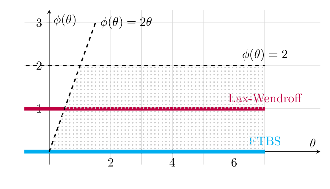
Fig. 9.4 \(\theta\)-\(\phi\) space for visualizing flux limieters. Two simple flux limiters,\(\phi\equiv0\) (blue) and \(\phi\equiv1\) (red) are sketched. These corresond with the FTBS and the Lax-Wendroff scheme. The hatched area shows the area where the TVD criteria from Equation (9.21) holds.

Fig. 9.4 shows the \(\theta\)-\(\phi\) space, where the area that ensures TVD is hatched. The area is bounded by the lines \(\phi(\theta)= 2\) and \(\phi(\theta)= 2\theta\).

We can now better understand where the oscillations in the Lax-Wendroff scheme comes from. As long as the slope \(\theta \ge\frac{1}{2}\), the scheme is inside the TVD regime. However, for negative or small values of \(\theta\) (\(\theta\le \frac{1}{2}\)), the red line, representing Lax Wendroff, is outside the hatched area that ensures TVD. It is for these small \(\theta\) that the oscillations start to grow.

A numerical scheme that has low values of \(\phi(\theta)\) will typically yield large numerical diffusion. The FTBS, where \(\phi(\theta)\equiv 0\), is one such example. If a numerical scheme is close to, or above the upper limit for TVD, the solution will, typically generate oscillations, such as in the Lax Wendroff scheme for small \(\theta\).

9.3.3. Classical TVD schemes

There exist many flux limiters that ensures \(\phi(\theta)\) falls within the area that guarantees TVD. The flux limiters characteristics depend on where in the TVD area they are located. A numerical scheme that has low values of \(\phi(\theta)\) will typically yield large numerical diffusion. The FTBS, where \(\phi(\theta)\equiv 0\), is one such example. If a numerical scheme is close to, or above the upper limit for TVD and have small values of \(\theta\) (i.e., steep slopes), the solution will, typically generate oscillations, such as in the Lax Wendroff scheme for small \(\theta\).

9.3.3.1. Sveby restricted TVD and Sveby flux limiter

To avoid large diffusion and risk of oscillations, Sveby restricted the TVD area by excluding the lower part and the upper left corner, as illustrated in Fig. 9.5. The yellow area is the Sveby restricted TVD area.

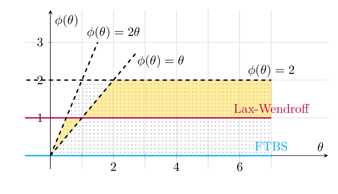
Fig. 9.5 \(\theta\)-\(\phi\) space for visualizing flux limiters. Two simple flux limiters,\(\phi\equiv0\) (blue) and \(\phi\equiv1\) (red) are sketched. These corresond with the FTBS and the Lax-Wendroff scheme. The hatched area shows the area where the TVD criteria from Equation (9.21) holds, and the yellow area represent the Sveby restricted TVD area.

The associated Sveby flux limiter follows the lower boundary of the Sveby restricted TVD area:

Sveby flux limiter

(9.22)\[\phi(\theta)=\text{minmod}(1,\theta)\]

9.3.3.2. Superbee flux limiter

The superbee flux limiter follows the upper boundary of the Sveby restricted TVD area:

Superbe flux limiter

(9.23)\[\phi(\theta)=\text{max}[0,\text{min}(1,2\theta),\text{min}(2,\theta)]\]

The superbee flux limiter is commonly used in ocean and atmospheric models, providing a scheme that has limited numerical diffusion. However, it can sometimes amplify gradients through anti-diffusion.

9.3.3.3. van Leer flux limiter

The van Leer flux limiter is designed to be roughly in the center of the Sveby restricted TVD area:

van Leer flux limiter

(9.24)\[\phi(\theta)=\frac{\theta+|\theta|}{1+|\theta|}\]

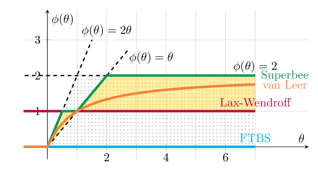
Fig. 9.6 \(\theta\)-\(\phi\) space for visualizing flux limiters. The colored lines represent the flux limieters: FTBS (blue), Lax-Wendroff (red), Superbee (green), and van Leer (orange). The hatched area shows the area where the TVD criteria from Equation (9.21) holds, and the yellow area represent the Sveby restricted TVD area.