8.7. Half-step schemes#
When we derived the McCormarck scheme in Section 8.6.1, we referred to the scheme as a predictor-corrector scheme. However, we also ended up using half time steps (\(t^{n+1/2}\)) to get to the final numerical solution. Schemes that incorporate half-steps in time or space, may also be referred to as half-step schemes. The Lax-Wendroff scheme is an interesting example to look into. We can derive the scheme in multiple ways, and one of them uses half-steps in both time and space. This two-step approach, is also referred to as the Richtmayer scheme. Below, you will see how this derivation looks like for the linear advection equation. However, the method can be extended also to other non-linear hyperbolic partial differential equations.
8.7.1. The Lax-Wendroff 2-step scheme#
When deriving the Lax-Wendroff scheme using the 2-step approach, we compute \(u_k^{n+1}\) using not the time derivative at \(t=n\Delta t\), but that at the half-step, \(t=n\Delta t + \Delta t/2=(n+1/2)\Delta t\), using a forward in time approach.
To obtain the spatial derivative at the half-time step, we must have the function values at \(t^{n+1/2}\), which we derive in the same way
The Lax-Wendroff method thus involves two steps:
Step 1: Calculting \(u\) at the half-steps in time and space
First, compute \(\frac{\partial u}{\partial x}\mid_{m,n+1/2}\) using central differences, that involve the mid-points \(m+1/2\) and \(m-1/2\):
Step 2: Calculate \(u_m^{n+1}\) using the half-step solutions from step 1
Compute \(u_m^{n+1}\) using the spatial derivative at \(n+1/2\):
For the linear advection equation, it is possible to merge step 1 and step 2, by inserting the expressions for \(u_{m\pm 1/2}^{n+1/2}\) from (8.23) into step 2 ((8.24)). After some massaging of the expression, you will end up with the same Lax-Wendroff scheme as we find in other derivations:
8.7.1.1. Application: propagation of top hat function using the Lax-Wendroff 2-step approach#
We apply the Lax-Wendroff scheme to the top hat initial condition.
The Lax-Wendroff scheme is implemented in the following Python function:
In the next code snippet, we set the discretization parameters and integrate the initial condition with the Lax-Wendroff scheme:
Number of time steps = 30
Number of grid points = 100
Time step = 0.010000
Grid size = 0.010000
CFL number = 0.750000
The solution at the end of the integration is shown below:
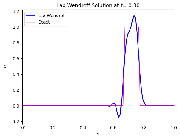
The Lex-Wendroff scheme avoids the excessive numerical diffusion of the Upwind scheme, but oscillations are still visible at the sharp transitions of the top hat function. These oscillations are known as the Gibbs phenomenon.